Mastering VLOOKUP Across Multiple Excel Workbooks
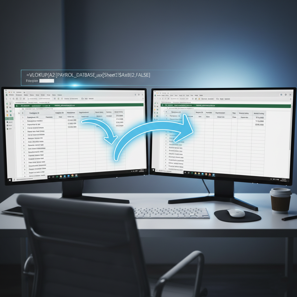
VLOOKUP is a cornerstone of data analysis, but many users struggle when the information they need isn’t just on another sheet, but in an entirely different file. Pulling data across workbooks is a powerful skill that allows you to keep your master files clean while tapping into large external databases.
In this guide, based on the tutorial by Maxwell Stringham, we will walk through the exact steps to link two workbooks using VLOOKUP, ensuring your data is accurate and professional.
Step 1: Prepare Your Workspace for Success
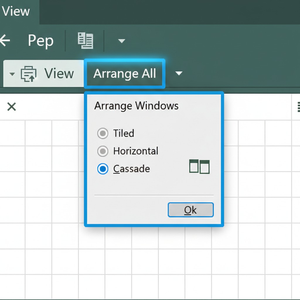
Before typing a single formula, the most intentional step you can take is to arrange your files so you can see them both at once.
- Arrange Vertically: Open both workbooks, then navigate to the View tab, select Arrange All, and choose Vertical.
- The Benefit: This allows you to easily click between files to select ranges without losing track of your formula progress.
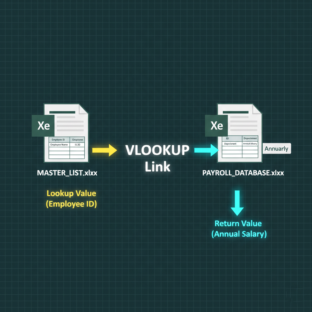
The Cross-Workbook Formula Breakdown
When writing a VLOOKUP that jumps between files, the syntax becomes a bit more complex because it must include the external file name.
The 4 Arguments of a Cross-Workbook VLOOKUP:
- Lookup Value: The common key in your current workbook (e.g., an Employee ID).
- Table Array: Instead of selecting a range in your current sheet, click over to the other workbook and highlight the entire table.
- Note: Excel will automatically add the filename in brackets (e.g.,
[FileName.xlsx]) followed by an exclamation mark.
- Note: Excel will automatically add the filename in brackets (e.g.,
- Column Index Number: Count the columns in the source table. If the data you want is in column I, that is the 9th column.
- Range Lookup: Always use FALSE for an exact match to ensure you aren’t pulling “close enough” data like rounded salaries.
Applying and Formatting the Data
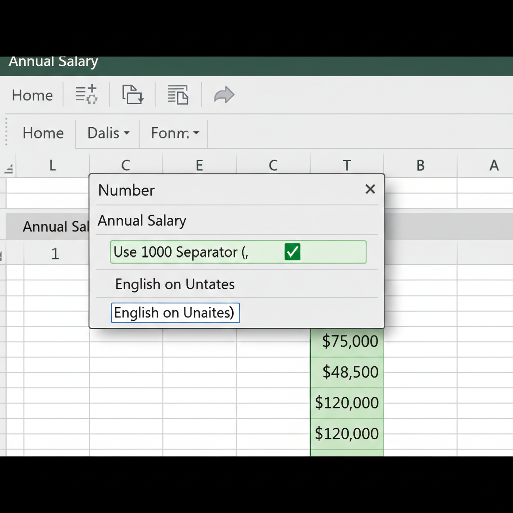
Once you have successfully pulled the first piece of data, you need to apply it to the rest of your list.
- Relative References: Use the fill handle (the small black plus sign in the corner of the cell) to drag the formula down. This adjusts the lookup value for each row while keeping the external table reference steady.
- Consistency in Formatting: Often, the pulled data won’t match the style of your master sheet. Select your new data, go to the Home tab, and use the Number formatting options to apply currency or thousand separators so it matches your source perfectly.
Important Considerations
When working across workbooks, remember these “cautious” tips:
- File Paths: If you move or rename the source file, the link may break.
- Open vs. Closed: VLOOKUP generally works best when both workbooks are open during the initial setup.
- The “Leftmost” Rule: As with all VLOOKUPs, your lookup value (the ID) must be in the first column of the range you select in the external workbook.
Bridging the Data Gap
Using VLOOKUP across multiple workbooks is a game-changer for anyone managing segmented data. By arranging your windows vertically and carefully selecting your table array from the external file, you can build dynamic reports that update effortlessly.


Leave a comment