Mastering VLOOKUP in Excel: The Ultimate Beginner’s Guide

If there is one Excel function that separates the beginners from the pros, it’s VLOOKUP. Short for “Vertical Lookup,” this function allows you to search for a specific value in one column and return information from another column in the same row.

In this guide, based on the expert tutorial by Kevin Stratvert, we will break down how to use VLOOKUP, how to avoid common pitfalls, and why you might eventually want to upgrade to its modern successor, XLOOKUP.

What is VLOOKUP?

VLOOKUP is designed to find data in a vertical list. Imagine you have a customer ID and you need to find that customer’s name in a massive database. Instead of scrolling, VLOOKUP does the heavy lifting for you.

The 4 Arguments of VLOOKUP:

1. Lookup Value: The piece of data you already know (e.g., the Customer ID).
2. Table Array: The range of cells where the data lives.
3. Column Index Number: The column number in the table from which to retrieve the data (e.g., Column 2 for “Name”).
4. Range Lookup: Enter FALSE for an exact match or TRUE for the closest match.

The Golden Rules of VLOOKUP

Before you start typing formulas, you must structure your data correctly to avoid errors:

• The Leftmost Rule: The value you are looking up must be in the leftmost column of your table array.
• Format as a Table: Use Ctrl + T to turn your data into an official Excel Table. This makes your formulas dynamic—if you add more rows, the VLOOKUP will automatically include them .
• Sorting: If you are using a “Closest Match” (Range Lookup = TRUE), your lookup column must be sorted in ascending order.

Exact Match vs. Closest Match

Most users need an Exact Match. If you search for Customer ID #4, you only want the data for #4. If it doesn’t exist, Excel will return an #N/A error.

However, Closest Match is perfect for scenarios like tax brackets or shipping incentives. For example, if a customer orders 26 cookies and your discount tiers are at 0 and 100, a closest match VLOOKUP will “fall back” to the 0 tier to give the correct percentage.

Cleaning Up with IFERROR

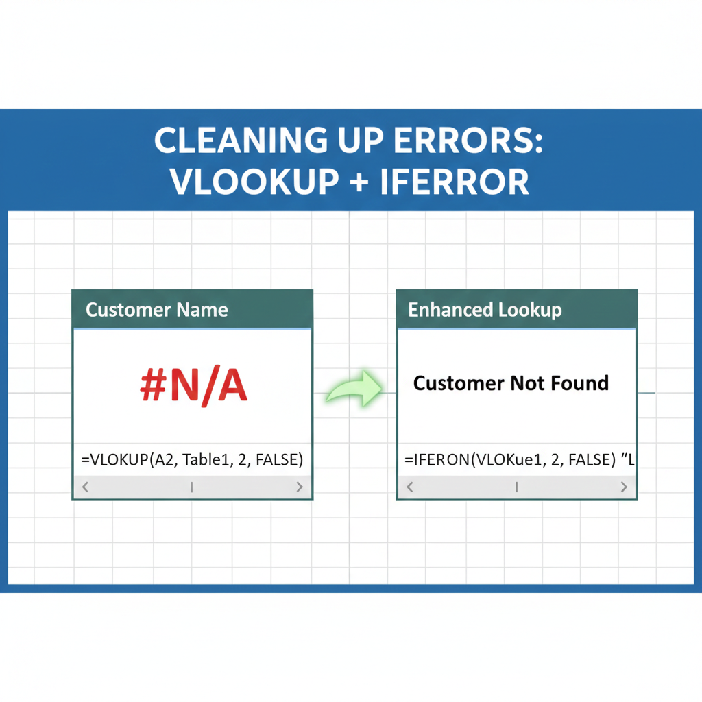
Nothing looks less professional than a spreadsheet full of #N/A errors. You can wrap your VLOOKUP in an IFERROR function to display a friendly message like “Not Found” instead.

=IFERROR(VLOOKUP(...), "Not Found")

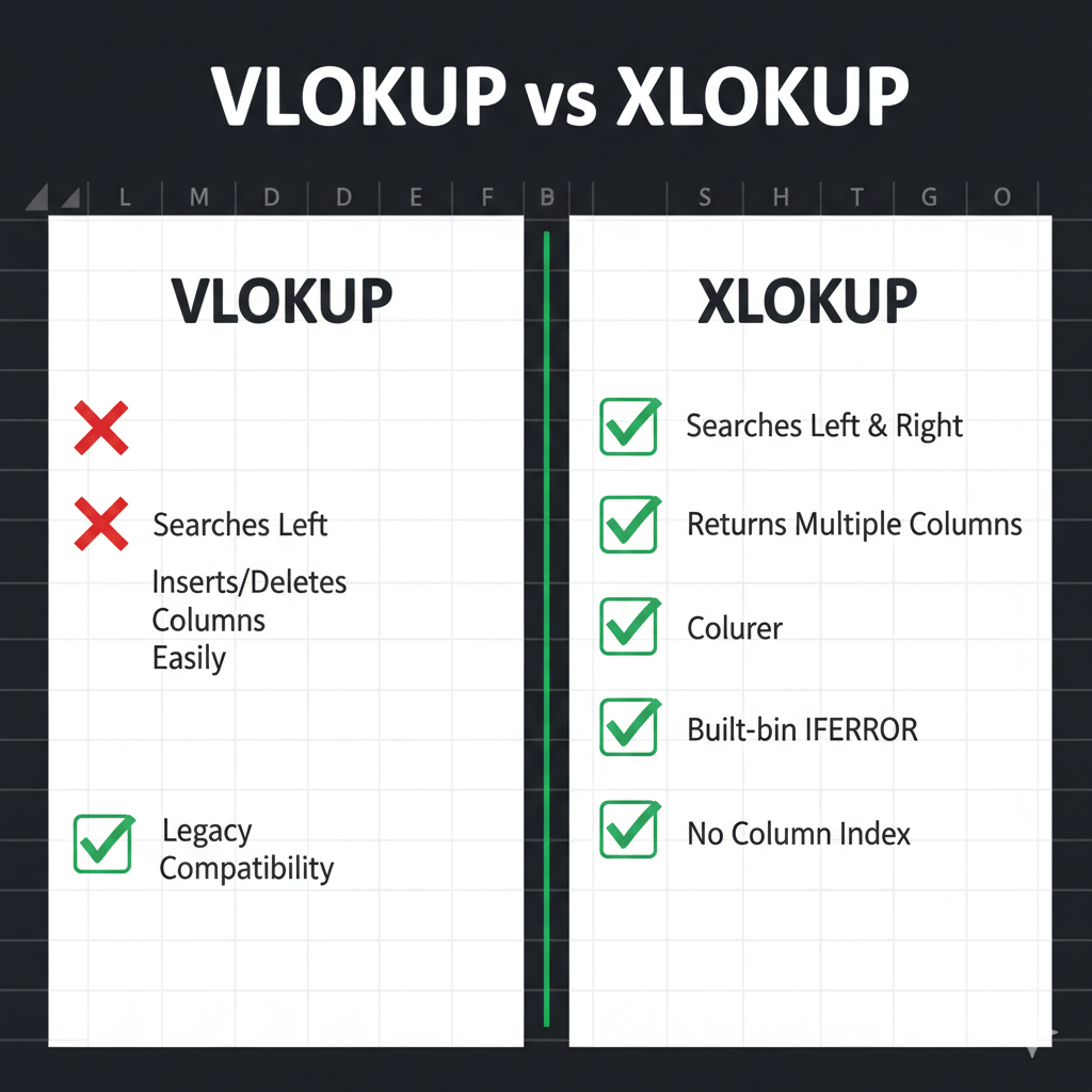
The Next Level: XLOOKUP

While VLOOKUP is legendary, it has limitations—it can only look to the right, and it requires specific column index numbers.

XLOOKUP is the modern replacement that solves these issues.

• Look Left or Right: Your lookup value no longer has to be in the first column.
• No Column Numbers: You simply select the column you want to search and the column you want to return.
• Built-in Error Handling: XLOOKUP has an “If not found” argument built right in, so you don’t need the extra IFERROR function.

Which Should You Use?

If you are working on a modern version of Excel, XLOOKUP is almost always the superior choice. However, understanding VLOOKUP is essential for maintaining older spreadsheets and collaborating with others who may not have the latest updates.

Mastering these lookups will save you hours of manual work and turn you into an Excel power user.