VLOOKUP in Excel: Your Ultimate Guide to Smarter Data Analysis

If you use Excel, you need to know VLOOKUP. It is arguably the most used function in the program because it allows you to automate data analysis, save massive amounts of time, and—most importantly—avoid the manual entry errors that plague complex spreadsheets.

In this guide, inspired by Leila Gharani’s expert tutorial, we will walk through exactly what VLOOKUP is, how to use it across different sheets, and how to fix those pesky errors that stop your work in its tracks.

What is VLOOKUP and How Does it Work?

VLOOKUP stands for “Vertical Lookup.” Its primary job is to find related information from one place and bring it over to another.

Imagine you have a customer name and need their profession. Instead of manually searching through thousands of rows, VLOOKUP does the work for you.

The 4 Pillars of a VLOOKUP Formula:

1. Lookup Value: What are you searching for? (e.g., a Customer Name).
2. Table Array: Where is the data range that contains both the lookup value and the answer? .
3. Column Index Number: Which column number holds the answer? (Excel starts counting from the left as “1”).
4. Range Lookup: Use FALSE (or 0) for an exact match, or TRUE (or 1) for a closest match .

Looking Up Data from Another Sheet

Often, the data you need isn’t on the same page. VLOOKUP handles this easily:

• Start your formula as usual.
• When it’s time to select the Table Array, simply click onto the other sheet and highlight your data.
• Pro Tip: Always use the F4 key to “fix” your range (adding dollar signs like $A$2:$B$10). This ensures that if you drag the formula down, the data range doesn’t shift.

Exact Match vs. Closest Match

• Exact Match (FALSE/0): Use this for IDs, names, or specific codes. If the value isn’t there, you want to know about it.
• Closest Match (TRUE/1): This is perfect for ranges, like tax brackets or grading scores. For example, a score of 75 might fall into a “C” grade range.
  • Important Rule: For a closest match to work, your lookup values must be sorted in ascending order.

Troubleshooting Common VLOOKUP Errors

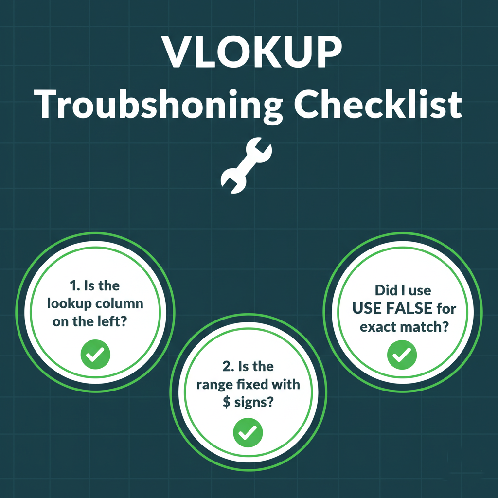
Even pros run into issues. Here are the three most common VLOOKUP “Gotchas” and how to fix them:

1. The Leftmost Rule: VLOOKUP can only look to the right. Your lookup value (the thing you know) must be in the leftmost column of your selected range.
2. Sneaky Spaces: If your VLOOKUP returns an #N/A but the value looks correct, check for hidden spaces. You can wrap your lookup value in the TRIM function to clean these up automatically.
3. The #N/A Cleaner: If a value truly doesn’t exist, use the IFNA or IFERROR function to replace the ugly error message with something friendly like “Not Found”.

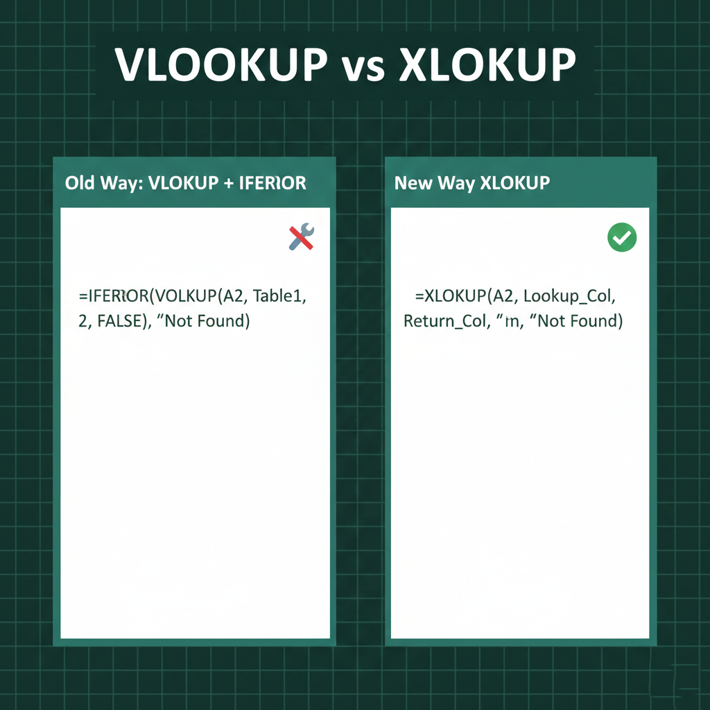
Future-Proofing: Meet XLOOKUP

While VLOOKUP is the “OG” function that works in all versions of Excel, users with Microsoft 365 should check out XLOOKUP. It removes the “leftmost” restriction and handles errors even more elegantly.

Automate Your Workflow Today

Mastering VLOOKUP is a major milestone in your Excel journey. By understanding how to fix your ranges and handle errors, you turn hours of manual cross-referencing into seconds of automated magic.